

Overview
This section of notes explains how strain, piezoelectric and pressure gauges operate and how to utilise them in a circuit for the best results.
Objective
- To understand the principles of operation of various force and pressure sensors.
- To be able to design some simple signal conditioning circuits for these sensors.
Study Time: 4.0 hours

Basic Principles
The parameters of pressure and acceleration are grouped with force as they are linked to that parameter.
For example a pressure P acting on a surface A exerts a force F = PA on that surface.
Also, a known mass M, when subjected to an acceleration Ÿ, experiences a force of F = M Ÿ. Thus measurement of the force allows the pressure or acceleration to be estimated.
Of the principles employed in force estimation, two of the most important are (a) strain gauge methods, and (b) piezoelectric methods.
Strain Gauges
A strain gauge (SG) consists of a long, thin, metal wire or foil packaged in a compact manner and affixed to a carrier The carrier in turn is glued to some element which is exposed to the unknown force and which experiences a strain due to it.
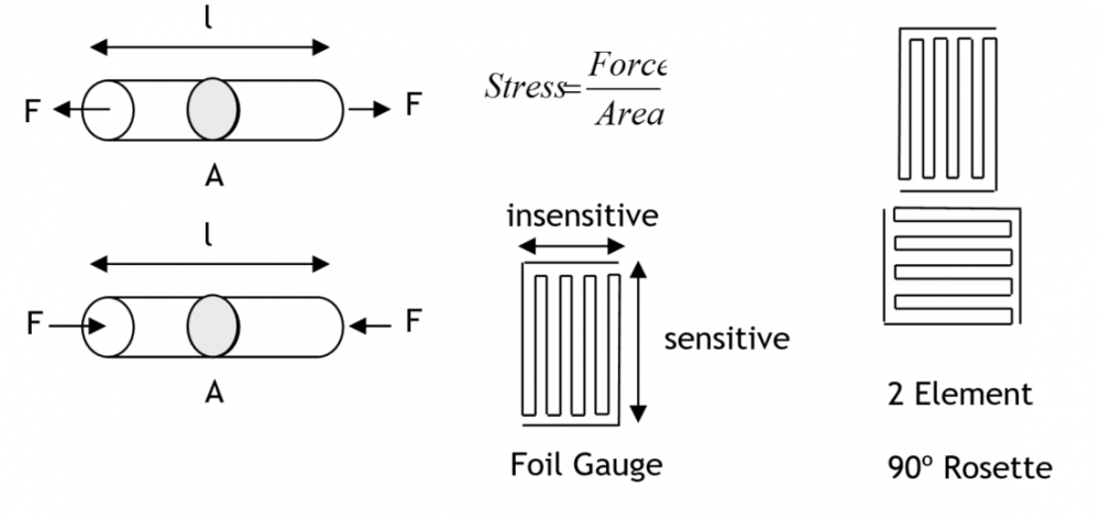
Strain is defined by the following equation:
Where ε is the strain, dimensionless, delta l is the change in length of the object and l0 is the resting length of the object. The strain gauge therefore shows the amount of strain and therefore stress that is incident on the material.
As the SG element is glued to the element under stress, the strain experienced by the element is also experienced by the SG. The unstressed resistance of the SG wire or toil is given by:
where ρ is the resistivity of the gauge material, l is its length and A is its cross-sectional area.
When under tensile stress the resistance becomes:
From which it can be shown that the proportional resistance change is linearly related to the strain i.e.
where K is the gauge factor which depends on the gauge material.
The same argument applies to compressive strain except that a reduction in resistance is experienced rather than an increase.
Strain gauges are used in two forms, wire and foil. The basic characteristic of each are the same. The design of the SG itself is such as to make it very long, to give a large nominal resistance, and to make the wire or foil very fine such that it possesses negligible strain resisting qualities in itself. Finally it is necessary to make the gauge of a unidirectional nature so that it responds to strain in only one direction. The material is folded to achieve a long high resistance length in a compact form. If a strain is applied at right angles to the intended direction, the gauge will tend to unfold with no change in resistance. Nominal SG resistances lie in the range 60, 120, 250, 350, 500 and 1000Ω.
Because the SGs are constructed from metals such as nickel, chromium and their alloys, they demonstrate positive coefficients of resistance change with temperature, and so SG circuits have the potential to generate temperature dependent signals which could swamp the strain-related signal. The solution to this problem is provided by the inclusion in the measurement of a second ‘dummy’ gauge as closely matched to the active gauge as possible (see 2-plane rosette above). This dummy gauge is not included to have any part in strain measurement but merely for temperature compensation. The dummy gauge is fixed to the sample as is the active gauge, but it is aligned along the insensitive axis. Thus it gives no output due to strain but any change in the active gauge, due to temperature change, is matched by the dummy.
Strain Gauge Interface Circuits
The relative change in resistance obtained from a gauge is small, typically 0.2% full scale. This indicates that the output signals to be expected from strain gauge-based systems will be low and considerable amplification will be necessary.
A simple potential divider incorporating a gauge will provide
It is clear that at no load (X=0) this circuit output is 0.5Vin, whereas for a maximum gauge resistance change, x, of say 0.2% (=0.002), the output is 0.5005Vin.
This in effect means that the maximum signal magnitude is 0.5x10⁻³ Vin "sitting” on top of a dc voltage of 0.5 Vin.
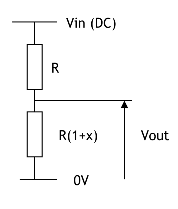
Fig 1. simple potential divider
Some means must be found to amplify the signal component while not amplifying the dc component. It is not possible in most cases to employ a blocking capacitor for the dc component as the signal bandwidth will extend all the way down to dc. The solution is to set up a second potential divider which will produce a second dc component which can be used to cancel the first.
The double potential divider is known as a quarter bridge (Figure 2) and the cancellation of the common mode component is performed by a differential amplifier, more particularly an instrumentation amplifier.
If R1 = R2 = R3 = R
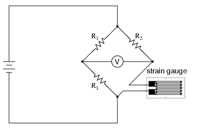
Fig 2. Quarter Bridge Strain Gauge Circuit
Insensitivity to temperature variation for the system of Figure 2 is achieved by introducing a second inactive gauge for "R2" (Figure 3). This gauge is bonded to the test piece in the vicinity of the active gauge but its orientation is such that it is not strained; however it experiences the same temperature variation as the active gauge and will change resistance accordingly. A temperature change therefore causes a common mode voltage change at the bridge output terminals and not a differential voltage change.
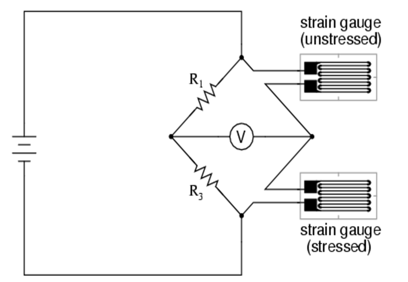
Fig 3. a quarter bridge strain gauge circuit with temperature compensation
SGs provide relatively low-level output signals; the signal levels to be expected are often described by the system sensitivity. Consider for example Figure 1, with a gauge with a maximum resistance change, x, of 0.2% corresponding to a maximum output of 0.5x10⁻³ Vin. If Vin is 5V the max output will be 2.5 mV. The system sensitivity is then quoted as 0.5mV/V.
For a given type of gauge system, sensitivities can only be increased by increasing the number of active elements in the bridge; which is only possible in certain applications.
Figure 4 shows a bridge with two active elements which has double the sensitivity of the single element case.

Fig 4. Use of two active strain gauge elements to double sensitivity
Figure 5 demonstrates a further doubling achieved by a full bridge in which every element is active. This maximum sensitivity system can be realised in applications where free access can be had to a component under simultaneous compressive and tensile stresses.
An example of such an application is a cantilever in which the upper section is in tension while the lower section is in compression. See http://www.rdpe.com/ex/hiw-sgpt.htm for a good description of how this works.
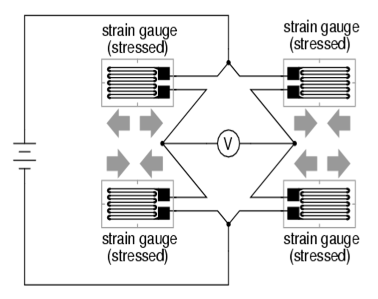
Fig 5. Full bridge Strain Gauge circuit
Notice that in all of these cases the bridge output is essentially non-linear, although a close approximation to linear operation is achievable over a limited range.
It should be remembered from circuit analysis that the equation governing the behaviour of Wheatstone bridges is:
Where Zn refers to the corresponding resistor, Vo is the output voltage and Vs is the supply voltage.
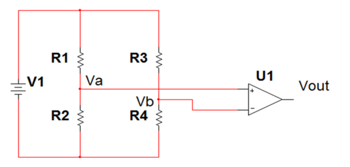
Strain Gauge Full Bridge Sensitivity Calculation
Example:
No strain: R1 = R2 = R3 = R4 = R, Va = Vb and U1 output = 0V
Strain: R1 and R4 "x" compressed, R2 and R3 "x" stretched
Bridge Excitation
Gauges may have a resistance as low as 60 ohms; they may be incorporated in a bridge, which is fairly remote from the amplifier so good output signal levels demand a high excitation voltage.
The source of bridge excitation should ideally be very stable as any variation will be coupled to the amplifier input. If the bridge is perfectly balanced then this variation will appear as common mode and be rejected; however if there is bridge imbalance a proportion of any excitation variation will appear as a differential mode signal and be amplified by the SG amplifier.
SG Amplifiers
For non-demanding applications, op-amps connected as differential amps can be used as bridge amplifiers, however, the common mode rejection (CMR) of such an arrangement will depend on the balancing of the bridge. This shortcoming is overcome by using specialist instrumentation amplifiers (Fig 6).
The amplifier bandwidth can be restricted to match the low mechanical loading bandwidth. This will improve interference suppression and increase the signal to noise ratio, thus improving measurement accuracy.
The advantages of an instrumentation amplifier include:
- Very high input impedance (inputs draw essentially no current)
- Very low offset (0V in = 0V out)
- Very high open loop gain
- Very high common mode rejection ratio (only difference signals are amplified)
- Closed loop gain is set by a single resistor (Rgain)
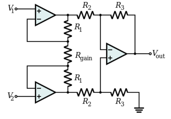
Fig 6 instrumentation amplifier
Piezoelectric Methods
A piezoelectric material is one in which an electric potential appears across certain surfaces of a crystal if the dimensions of the crystal are changed by the application of a mechanical force. (For these materials the opposite effect also occurs, i.e. if a potential is applied between opposite faces of a crystal it will change its physical dimensions – this is the basis for ultrasonic transducers).
Piezoelectric materials occur naturally e.g. quartz, tourmaline, but the most efficient piezoelectric materials, such as barium titanate and lead zirconate titanate, are synthetically produced. Particular directions of polarisation can be introduced at manufacture.
Pressure applied to the crystal produces a certain force over the area of the crystal. The crystal deforms mechanically and a proportional charge is produced within the crystal. Consequently a voltage is generated across the faces of the crystal of a value dependent on the crystal dimensions, as the crystal impedance is essentially capacitive.
where v is the open circuit voltage across the crystal, q is the charge produced by the piezoelectric material, and C is its capacitance.
Piezoelectric Interface Circuits
As the pressure or force-related signal produces a charge within an essentially capacitive transducer, there are two basic approaches to the interfacing task. In the first of these the crystal is presented with a very high (ideally infinite) input impedance amplifier which will preserve and amplify the consequent voltage (V=Q/C); this is the voltage amplifier approach. Alternatively the crystal is presented with an amplifier having a very low (ideally zero) input impedance which will encourage any charge produced within the crystal to flow into it where it can be accumulated (and therefore measured) by integration. The amplifier in this latter approach is known as a charge amplifier.
Fig 7 illustrates the loading of the crystal with a unity gain buffer as an example of the voltage amplifier approach. In a practical circuit the input signal must be protected from external interference by the use of a coaxial cable with an earthed screen. This, in effect, places a cable capacitance Cc in parallel with the crystal capacitance Ca. Also a resistor Rb must be provided at the amplifier input as a path for DC bias current.
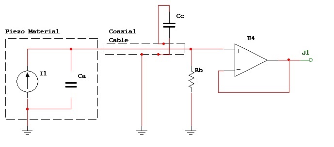
Fig 7. Voltage Amplifier Approach
Calculations show that this circuit has a low cut off frequency ω = 1/Rb(Ca+Cc) rad/s. For signals above this frequency the o/p voltage is given by vo = va.Ca/(Ca+Cc). Thus the cable has the effect of reducing the accelerometer sensitivity.
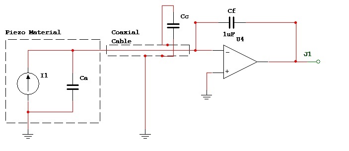
Fig 8. Charge Amplifier Approach
Figure 8 shows the crystal model connected to a charge amplifier. Again Cc represents the cable shunt capacitance and Rf is included in the feedback network as a path for dc bias current. For signals above a low cut off frequency of 1/RfCf rad/s the current is integrated in Cf to provide an o/p voltage vo = va.Ca/Cf. Notice how this arrangement is not affected by the cable capacity and how Cf provides a convenient method of changing the gain.
Accelerometer
The most common way for a piezoelectric transducer to be used is the piezoelectric accelerometer. This is shown in Figure 9.
- The mass experiences an inertial force which is proportional to the acceleration. The force is measured by applying it to a piezoelectric crystal.
- The signal amplitude for a given acceleration depends on the sensitivity of the accelerometer.
An unknown force, which could be due to a pressure or acceleration may be made to bear either on an elastic structure (such as a cantilever) or a membrane on which is mounted a strain gauge or piezoelectric crystal. In the case of acceleration, a specialist transducer known as an accelerometer contains a known inertial mass which experiences a proportional inertial force when exposed to the unknown acceleration. The force in turn may be estimated by applying it to a piezoelectric crystal.
Piezoelectric accelerometers are very robust, but cannot be used for slow varying or constant acceleration measurements because of their frequency response. The signal amplitude for a given acceleration depends on the sensitivity of the accelerometer. Both charge and voltage sensitivities are normally specified.

The charge sensitivity of an accelerometer is defined as the amount of charge (typically in pC) that is produced per unit of acceleration i.e.
typical units are mV/(m/s2)
Task 1
Modern accelerometers are called Micro-ElectroMechanical Systems (MEMS)
Some MEMS devices use piezoelectric transducers as described above, others use different transducers. Which other transducers would be suitable and how would they work in this application?
Pressure Gauges
A third type of widely used transducer are pressure gauges. Pressure is measured using a number of different units: psi (pounds per square inch), Pascals (Newtons per square metres), Bars, Torrs, mmHg (millimetres of mercury) etc., with Pascals being the Standard International (SI) unit.
There are essentially three different pressure measurement types:
- Gauge pressure: this is the pressure measured with reference to the local atmospheric or ambient pressure. Transducers such as tyre pressure gauges measure gauge pressure.
- Absolute pressure: this is the pressure measured with reference to zero pressure. Instruments measuring atmospheric pressure, e.g. Bourdon Gauge, Aneroid and Mercury Barometers etc. measure absolute pressure.
- Differential pressure: this is the pressure measured with reference to another pressure, e.g. on either side of an orifice plate in a pipe.
Devices for measuring pressure include:
-
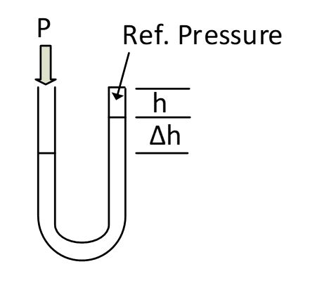
Manometer. Works on the principle of Pressure = density x gravity x height. Simple and accurate, but with poor resolution (due to surface meniscus).
Not robust and requires an additional sensor to enable electronic reading to be obtained.
Can measure absolute (reference vacuum), relative (open ended at one end) or relative (pressure applied both ends) pressure.

- Bourdon Tube. Works on the principle that applied pressure causes the tubular coil to uncurl and amount of uncurling is proportional to pressure.
The most commonly used pressure measurement instrument. Good resolution and accuracy, but not very robust and rather large.
- Differential Pressure cells. These work on the principle of having a diaphragm which is distorted by applied pressure and the distortion can be measured by a strain gauge or similar. There are also piston types available.
The most commonly used sensor for electronic sensing of pressure. Small, robust, accurate.

Piston pressure sensor
Summary
In this section we have looked at the principles of operation of some sensors for measuring force, pressure and acceleration. We have also examined signal conditioning circuits for these sensors to improve measurement linearity, accuracy and resolution.
References
Morris, Alan S. (2001) Measurement and Instrumentation Principles 3rd edition, Oxford: Butterworth-Heinemann (ISBN 0-7506-5081-8)
National Instruments Website http://www.ni.com/tutorials/ [21/06/17]
Sensorland Website http://www.sensorland.com/ [21/06/17]