
Introduction
This lesson shall introduce the use of arrays in the LabVIEW development platform. An array is a data structure in programming consisting of a collection of elements, all of which are of the same data type. Each element in an array is indexed by some method so that specific elements can be referenced from within the array data structure.
This lesson shall also introduce the use of graphs and how they vary to charts in LabVIEW.
Finally, this lesson shall demonstrate how to write data to an external file, in our case using an MS Excel spreadsheet file for illustrative purposes.
To summarise, this lesson shall cover:
- How to manually create an array in LabVIEW
- How to have LabVIEW create an array using a loop structure
- How to manipulate Arrays using LabVIEW Array Functions
- How to plot graphs in LabVIEW.
- How to read and write array data into an external spreadsheet
Arrays
As noted in the introduction, an array is a data structure that consists of a collection of elements of the same data type. Each element in an array is indexed, i.e., it has a referenceable address within the array. Each array therefore can be defined in terms of:
- Its elements – the contents of the array.
- Its dimensions in terms of length, height, depth, etc. that can be referenced in the form of an address.
An array can be one-dimensional or multi-dimensional. Arrays are used to store elements of the same data type, e.g., numeric, string, etc. and become useful when working with large collections of similar data that are to be processed in a similar manner.
In LabVIEW, arrays are referenced using a zero-based index; the first element being at location 0 in the array and the nth element being at location n-1. For example, if a class list were stored in a one-dimensional array of ‘string’ data type it could take the following form:
|
Index |
0 |
1 |
2 |
3 |
|
Elements |
“Sarah” |
“Billy” |
“John” |
“Susan” |
Manually Creating an Array in LabVIEW
To manually create an array in LabVIEW, first an array shell must be placed on the Front Panel. This array shell can then be populated with the elements of a suitable data type.
To place the array shell, select ‘Controls Palette >> Data Container >> Array’ and left click on the front panel to place the object.
The array shell can then be populated with a specific element type by dragging and dropping that control or indicator object into the shell body.
You can build arrays of numeric, Boolean, path, string, waveform, and cluster data types.
Note: an array shell that has not been populated with elements cannot be wired to from within the Block Diagram.
Note: if the programmer attempts to populate the shell with invalid objects (e.g.: a graph) LabVIEW will not allow the object to be placed within the shell.

Figure 1: Array Shell Object

Figure 2: Dragging a data type into an array, e.g., a numeric indicator

Figure 3: An array populated with numeric data
An array can be expanded by dragging the physical dimensions of the array shell using the Positioning Tool.
To add an additional dimension to the array, right click the array index and select ‘add dimension’.
Note that the indexes operate by showing the user the value at the indicated address within the array, see illustration.
- Array Element
- Row Index
- Column Index

Figure 4: A 2 by 4 array with column and row indices illustrated

Figure 5: The Same 2 x 4 array showing value at indexed address
Exercise 1: Creating an Array Using a Loop Structure
A simple method for creating an array is to use a loop to populate the array with data and automatically index each element in the array using the value of the loop iteration.
First place an array shell on the front panel and populate it with a numeric indicator object. Note that as it has been populated with an indicator object, the wiring terminal on the Block Diagram will be on the left hand side of the array block.

Next, create a simple FOR loop in the block diagram:
- Place a FOR loop in the Block Diagram (leaving the array object outside the FOR loop structure).
- Create a Constant control for the FOR loop count and set the value to 4. Note: right-click on the loop count terminal and select ‘Create Constant’.
- Place a ‘Random Number (0-1)’ function within the loop and wire to the array block.
Note that the object identified by (4) is called the ‘loop tunnel’.

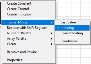
In the latest version of LabVIEW auto-indexing is set by default when wiring a loop to an array. To check that auto-indexing is selected, right-click the tunnel block on the FOR loop’s border and select ‘Tunnel Mode >> Indexing’.
Note that if auto-indexing is disabled the tunnel can either pass the last value, a concatenated value, or a conditional value out of the FOR loop. This might be useful when the programmer wants to extract a specific value from a set of loop-generated data.
On the Front Panel:
- Expand the array to confirm that each element is set at zero or null value.
- Now execute the VI by pressing the RUN button in the LabVIEW toolbar.
Check that the array has been populated with random numbers, each being applied to a new element in the array.

Multi-dimensional Arrays
Note that the default array created by a loop structure is a one-dimensional row array. Embedding a FOR loop inside a second FOR loop could be used to populate a two-dimensional array.

Figure 6: Block Diagram

Figure 7: Front Panel
Manipulating Arrays using LabVIEW Array Functions
LabVIEW provides several tools for analysing or manipulating arrays, these are commonly termed ‘Array Functions’ and can be found in ‘Functions Palette >> Array’ from the Block Diagram. Some of the most common array functions are described below:
- Array Size – Returns the number of elements in each dimension of the array.
- Initialise Array – Creates an n-dimensional array in which every element is initialized to the value of element.
- Build Array – Concatenates multiple arrays or appends elements to an array.
- Array Subset – Returns a portion of array starting at index and containing a defined number of elements.
- Index Array – Returns the element or sub-array of an array at a defined location (the index). Can also be used to extract a row or column of a multi-dimensional array, i.e., to create a sub-array of the original.
There are many more array functions to explore. LabVIEW Help provides detailed descriptions of how each of these functions is used.
Exercise 2: Manipulating an Array Using Array Functions
This exercise shall provide a brief overview of some of the array functions noted in the previous section.
First, we need to manually create a two-dimensional array and populate it with numeric data.
- Drop an array shell into the Front Panel.
- Add a second dimension to the array (right-click the row index and select ‘add dimension’).
- Drag a numeric control into the array shell
- Expand the array to 2 x 4 by resizing the array shell
Set the numeric control to various values

Array Size
- Place the array size function on the Block Diagram
- Right-click the output terminal of the array size function and select ‘Create Indicator’.
Note that LabVIEW automatically creates an appropriate indicator type.
- On the Front Panel, RUN the VI and check that the array size function has correctly indicated the size of the array.

Build Array
- Place the build array function on the Block Diagram
- Resize the function to 3 inputs.
- Right-click the function and check that ‘concatenate inputs’ is selected
Note that by default, additional arrays are added onto a new dimension of the array.
- Wire the original array to input terminal 1.
- Right-click input terminal 2 and select ‘Create control’. On the Front Panel set the new array to any identifiable values.
- Right-click input terminal 3 and select ‘Create constant’. On the Block Diagram set the constants values also.
- Right-click the output terminal of the array size function and select ‘Create Indicator’.
- On the Front Panel, RUN the VI and check that the updated array consists of the original array + appended arrays.

Array Subset
Note: in this exercise, connect the ‘array subset’ function to the location (Wiring Point) as illustrated.

- Place the array subset function on the Block Diagram
- Using input constants, set the inputs to [1, 3, 0, 2] as illustrated.
Note that these inputs imply:- From the address [row, column] = [1, 0]
- Create a sub-array of with 3 rows of depth and 2 columns in width.
- Right-click the output terminal of the array size function and select ‘Create Indicator’.

On the Front Panel, RUN the VI and check that the sub-array consists of the expected subset of values from the updated array generated previously.

Index Array
Note: Connect the index array to the same Wiring Point as above.
- Place the index array function on the Block Diagram
- Using input constants, set the inputs to [3, 2] as illustrated.
Note that these inputs imply:
- The element at address [row, column] = [3, 2] shall be referenced
Right-click the output terminal of the index array function and select ‘Create Indicator’.

On the Front Panel, RUN the VI and check that the Indexed Element correctly references the value at the selected address: [row, column] = [3, 2].

Graphs
In LabVIEW, graphs are usually used to illustrate array data in a plot against some other variable, such as their array indices. Note that in LabVIEW, graphs differ from charts in that they accept their data at one time and plot the full dataset at once, whereas charts are used to plot single data points as they are generated. The two most common form of graph are the waveform graph and the XY graph:
- The waveform graph is used to plot single-valued functions, such as f(x) = mx + C, whereby the result of the function f(x) is plotted against evenly distributed values of x, i.e., x = 0, 1, 2, 3,
Note that the waveform graph is commonly used to plot time varying waveforms sampled at regular intervals.
- The XY graph is used to plot any set of data, evenly sampled or otherwise. XY graphs accept a cluster data type, containing both an x-array and y-array, where the graph is formulated by a line connecting [x1, y1], [x2, y2], [x3, y3], etc.
Waveform Graph
Wiring a one dimensional array to a waveform graph indicator will be interpreted as a single-plot waveform. By default, the single-plot waveform presents each value in the array against an evenly distributed index (∆x = 1) starting at x = 0.
Place a waveform chart and waveform graph and STOP Button on the front panel and create the following Block Diagram.

When executing the VI, the user should be able to see each random number being plotted in real-time on the Waveform Chart. In contrast the waveform graph will remain unpopulated until the WHILE loop is terminated with the STOP button.

After pressing the STOP button an indexed array is passed to the waveform graph, which subsequently plots the dataset.
Note: remember to check that loop tunnelling mode is set to ‘Index’ as opposed to ‘Last Value’.
Also note that the Waveform Graph illustrated here contains the same data as the Waveform Chart generated in real-time. The difference in appearance is due to x-axis scaling.

Multiplot Waveform Graph
A multiplot waveform graph accepts a 2D array of values and handles each row of the array as a single plot.
To illustrate this, add a second set of random values to your previous block diagram with an additional offset value of 2. Wire both arrays to your waveform graph.
Note use the ‘Build Array’ function to concatenate the two separate 1D row arrays into a single 2D array as illustrated.

When executing the VI (terminating the WHILE loop using the STOP button) the 2D array is passed to the Waveform Graph, which subsequently plots the two sets of data.

Graph Customisation
Right-clicking on the Waveform Graph and selecting Properties opens a dialogue box that allows the programmer to change various appearance and formatting graph attributes:


File I/O
In programming languages ‘File I/O’ refers to the operations of passing data to and from external files. LabVIEW offers several functions to handle these operations, generally located in the ‘File I/O’ sub-folder of the Functions Palette. These functions include the capability to:
- Open and close external files
- Read and write data to external files or spreadsheets
- File management, e.g., to create, delete, move and rename files and folders within the native file directory
- Read and write ‘*.lvm’ file types, which are LabVIEW measurement files developed by National Instruments.
This lesson shall only give a brief overview the ‘Write to Measurement File’ function, which can be configured to export data to an MS Excel file.
Write Measurement File
Using the FOR loop as illustrated, a set of random numbers is generated and wired into the ‘Signals’ input of a ‘Write To Measurement File’ function.
Note that the Iteration Terminal is also sent to the input of the function to provide a reference value in the new file.

When placing the ‘Write To Measurement File’ function on the Block Diagram, a dialogue box is presented in which the programmer can configure various properties of the file that will be generated by this function.
Note that in this example, the default settings are generally suitable with the following configurations:
- The Filename and directory location is determined by the user.
- The File Format is set to Microsoft Excel (.xlsx)

Locating and opening the file in MS Excel, we can check that the VI has successful written the random values.

Exercise 3: Building a Datalogger
In this exercise, students are required to create an application in LabVIEW (starting from the Blank VI template) that will monitor the reading from a virtual thermometer taking 10 readings per second, plot the record on a graph in real-time as the VI executes and export the data to a MS Excel file once the user stops the program.
Note that the Front Panel should consist of:
- A Thermometer Control, which the user will vary as the VI executes to generate a variable temperature plot.
- A Waveform Chart, which will show the Temperature Record in real-time as the VI executes.
- A STOP button.

The Block Diagram should contain:
- A WHILE loop that is terminated by the STOP button control.
- A Time-delay function introducing a 100 millisecond delay.
- A Waveform Chart that shows the Temperature Record in real-time as the VI executes.
- A ‘Write To Measurement File’ function (outside of the WHILE loop) configured to write the file to an MS Excel file once the VI is terminated by the user.

If correctly implemented students should be able to:
- RUN the VI and see on the Waveform Chart indicates temperature varying with time (in accordance with the user manipulating the thermometer slider).
- Locate and Open the MS Excel file. In the spreadsheet, select the two columns of data and plot a scatter graph.
- Compare the two Waveform Charts (LabVIEW and MS Excel) to confirm that the data has been successfully logged.

Figure 8: Real-time Temperature Data (LabVIEW)

Figure 9: Exported Temperature Data (MS Excel)
Summary
This lesson has provided a brief introduction to arrays, graphs and the tools available in LabVIEW to create or manipulate them. This lesson also provided a basic introduction to the File I/O functions offered by LabVIEW and illustrated how such functions might be used to build a datalogger.
Note that for additional resources on either of these subjects please refer to the LabVIEW Detailed Help documentation such as: